 English (UK)
  Česky (CS)
 The order properties determining the industrial schedule
A set of batches in the schedule and their sequence primarily depend on numeral parameters of jobs in a working task. For simplicity, let us assume that jobs in a task are coincided with customer orders. In this case, each order has two main parameters for scheduling: a) directive due date in calendar days or hours and b) processing time in hours. Below two notions, which were proposed by author, are described for each order and are essentially applied in the paper.
Production Intensity
When criteria for an optimal plan to be performed are determined, in addition to process or economic factors, we also should take account of personal relations between responsible persons. There are two key courses of decision making i.e.: rational and psychological. As for the rational course, decisions are based on mathematically proven results while psychological course of decision making is substantially based on intuition and psychology of employees. A good production plan should be well-balanced between needs and wishes of all people involved into the production process.
People involved into the production process are all part of an extensive network of relations that can be considered as a certain psychological field. Each field, e.g., magnetic or electric has a quantitative characteristic that is called “intensity”. Similarly, a psychological field arising during production process can also be described quantitatively; this quantitative description is called the production intensity H [Mauergauz, 1999]. However, unlike physical fields, production intensity cannot be measured physically; it has no physical dimensions i.e. it is a dimensionless value.
Such dimensionless intensity of a psychological field (whether large or small) can only be estimated by comparison with another field or with another state of this field, e.g., at any other point of time. We face a natural question: how to calculate production intensity?
For the purpose of intensity quantification, let us take note of the fact that the situation in a production shop is mainly characterized by two factors i.e.: total time required for job completion and slack time. Please remember the so called dynamic priority rules described above that take account of these two factors. These rules include the Minimum Slack Time (MST), Critical Ratio (CR), and the Apparent Tardiness Cost (ATC) rules.
However, criteria calculated under any of these rules have substantial deficiencies. First, there is no way to determine the values of such criteria if the job due date has already expired by the start of planning. However, the most important thing is that the cumulative machine and personnel load resulting from different jobs cannot be determined using such criteria.
Unlike the above dynamic priority rules, we can determine production intensity values not only for each job, but for each machine and for the production shop overall. Production intensity for a certain machine will equal the sum of intensities for jobs awaiting processing on such machine; while production intensity for a production shop overall equals the sum of intensities for all jobs or, which is the same, for all machines.
The total time required to perform “top-to-bottom” plan targets is made of two values i.e. the production processing time, transfer time and changeover time. Slack time can be a positive or negative value or be equal to zero. Therefore, calculation relations used to determine production intensity should be different at different signs of slack time values.
Thus, for one i-job:
(1)
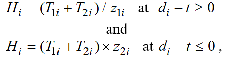
Where is the time duration determined by processing time pending at the time of planning; is the time component arising from the need to transfer jobs for further processing; is the production slack time in relation to plan targets; and is the tardiness from working task.
can be determined based on the following relation:
(2)
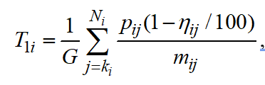
Where is the number of the first unfinished j-operation for i-job; is the total number of operations required to perform i-job; is the processing time of each remaining operation in hours or days; is the coefficient of readiness of j-operation (%); is the number of simultaneously processed items of i-job during j-operation; and is the average number of work hours or days in a planning period.
is calculated using the following relation:
(3)
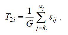
Where is the duration of required transportation and machine setup associated with j- operation for i-job.
Let's assume the following relation for dimensionless slack time available to a planning engineer:
(4)
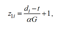
Where is the “psychological” coefficient of a given enterprise representing the level of "complacency” at available slack times or the level of “nervousness” if production due dates are failed to meet.
And, finally:
(5)
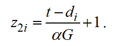
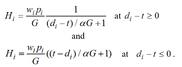
Similarly to the WSPT or ATC rules described above, intensity of a certain job can include a respective weight coefficient of priority . In particular, in the simplest case (where all readiness coefficients =0, the number of simultaneously processed items under one job =1, planning takes place for the first operation and all =1, while transportation and setup time can be ignored) intensity can be determined using the following formulas:
(6)
Now let’s consider the relation between intensity and available slack time or deadline tardiness (Figure 1).
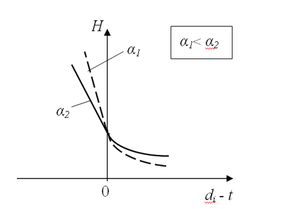
Figure 1. The relation between production intensity and slack time.
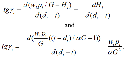
The slack time (difference between the due date for each job and the current time point ) is plotted on the X-line. On the positive part i.e. where , intensity values decrease hyperbolically as far as slack time increases. If slack time is negative i.e. there are tardiness on plan targets , intensity values increase linearly as far as tardiness increases. In expressions (4) and (5) if i.e. at the point of transfer from one relation to another, . Intensity values calculated using formulas (4) or (5) also coincide at this point. Besides, this point also sees the match of values for the following derivative:
which have been calculated been using both formulas. Thus, the straight line in the left-hand part of the chart is tangent at the transition point to the hyperbolic curve in the right-hand part of the chart.
Production intensity is dimensionless and has not any physical sense, but it has “psychological” sense. Really, increasing of production intensity grows anxiety for order completion. Figure 1 shows two curves for H changes; these curves differ by the value of “psychological” coefficient ; note that . As we can see, the greater is, the less intensity is associated with tardiness; however, the level of “relaxation” is also lower when slack time is available.
Dynamic utility function of order
We can use functions of the dynamic utility of orders V to evaluate whether it is possible and desirable to ensure a high level of customer service. Let’s assume that any order is quite useful for a manufacturer in a certain prospect. Note that the greater the order scope and order completion time is, the greater utility such order will have. In such a way, the possibility of order completion in future certainly has a positive utility and should yield a respective gain.
On the other hand, the closer the due date for an order is, a manufacturer starts facing certain difficulties. The utility value starts decreasing. However, if the manufacturer manages to perform the order when due, the order utility remains positive till the very time of order execution; and utility becomes zero at the time of completion. If the manufacturer fails to meet the due date, he usually gets into troubles with this. The order becomes the source of losses, thus, having a negative utility.
As we can see, if slack time is available for an order, a manufacturer generally counts on gain while in case of tardiness it incurs losses. The behavior of utility as a potential gain/loss function is described in numerous sources. Generally, all research results can be reduced to two options shown in Figure 2 [Mauergauz, 2016].
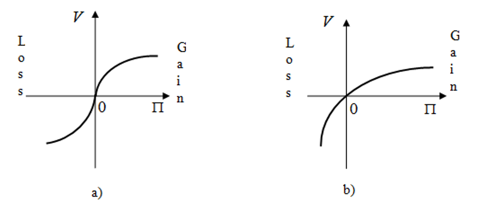
Figure 2. Charts of utility: potential gain/loss.
The gain value is plotted on the X-line (potential gain); the gain utility is plotted on the Y-line in the positive part of the X-line and the loss utility is plotted on the Y-line in the negative part of the X-line. The curve in Figure 2.a has been known as S-curve after well-know research of [Kahneman and Tversky,1984] that were awarded the Nobel Prize in the field of economics in 2002. Their research proved that people usually tend to take risks if there is a probability of potential loss (left-hand part of the chart in Figure 2.a). In this case, the concave left-hand part of the curve represents negative risk aversion - the second derivative has a positive sign at this interval of 2.a curve.
Unlike 2.a curve, 2.b curve always has a positive risk aversion no matter whether there is a probability of gain or loss. Please note that the chart of 2.b type [Grayson, 1960] was developed much earlier that 2.a chart. Differences between 2.а and 2.b curves probably arise from the pools of respondents and areas of money allocations. Studies Figure 2.a featured polls with low-income respondents whose income were insignificants and mainly used for personal consumption while studies in Figure 2.a dealt with large corporate investments.
Let’s use the above results of economic and psychological studies in order to build a function of dynamic utility of orders. Let’s assume that the current utility of i-order is as follows:
(7)
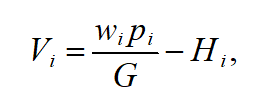
Where (as before) represents the processing time in days (hours) that remains before job completion; is the weight coefficient of priority; is slack time in days (hours) during the planning period; and is the production intensity associated with the order (job).
Let’s see how the dynamic utility function depends on slack time available till the established order due date (Figure 3) assuming that the orders has not yet been started i.e. does not depend on time.
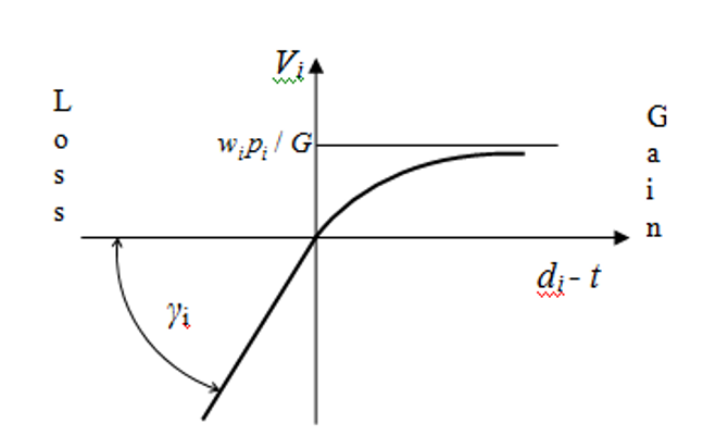
Figure 3. Dynamic order utility curve.
The depicted curve in the positive part of Figure 3 ( ) approaches the asymptote.
(8)
In the negative part ( ) the curve gets transformed into a straight line for which:
(9)
If we compare the curve in Figure 3 with the curves in Figure 2, we can see that the slack time available for a job determines gain or loss on Figure 3. The presence of an order is a substantial gain in a far prospect but the rate of gain growth decreases with the farness. In this part the behavior of the order utility function curve is absolutely similar to both curves shown in Figure 2.
The negative part of Figure 3 is similar to the loss part in Figure 2. In this part the curves in Figure 2 have different shapes. In order to check if the curve in Figure 3 is correct in the negative part, let’s assume human behavior as described above. As corporate managers use dynamic utility functions, their behaviour will be closer to the curve in Figure 2.b rather than 2.a curve as they are unlikely to take risks even in the loss part.
However, this is formally impossible to use 2.b curve as the order utility function as positive risk aversion typical of this curve results in a sharp increase of negative utility and, consequently, limits the potential loss value. The order utility function shall not have such a limit as, actually, any tardiness is possible during order execution. Therefore, the correct behavior will be a linear drop of the dynamic order utility function where risk aversion (the second derivative of the function) equals to zero. Figure 3 shows exactly this dependency.
Due to its additivity properties, both the production intensity and order utility for different orders can be added. Therefore, the average utility of the whole set of orders can be calculated.
If the number of order is at the planning horizon, their cumulative utility equals to the sum of utilities of each order as orders are generally independent. Orders, as a rule, are independent and the total value of the function of the current utility of orders:
(10)
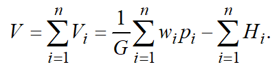
Value of function changes in time as the slack time available for a job is alternating. Besides, some orders are completed, and new orders arrive.